This chapter provides a detailed description of the Monte Carlo simulation methodology used in this paper, as well as the Monte Carlo simulation program MCSheild, and simplified arithmetic examples are provided for two typical nuclear facility scenarios in the dataset.
Introduction to the monte carlo method and program
Monte Carlo methods operate by calculating the statistical mean of an estimate as the solution to a problem. Monte Carlo methods were first applied in the testing and verification of nuclear weapons and played a crucial role in the U.S. Manhattan Project. In particle transport calculations, Monte Carlo methods can accurately describe 3D complex geometrical and physical reactions. Moreover, the convergence speed is independent of problem dimensionality, and computational errors can be easily discerned. In recent years, in the field of radiation protection, with the increasing demand for refined radiation shielding calculations, Monte Carlo methods and procedures have played an irreplaceable role in the simulation of full core refinement, shielding calculations, and shielding design optimization.
Tsinghua University Radiation Protection and Environmental Protection Laboratory developed MCShield20, which is a Monte Carlo software that is used for radiation shielding calculations. It simulates neutron, photon, and electron transport with parallel computations and effectively solves deep penetration and complex shielding problems in Monte Carlo variance reduction techniques. The software features robust pre- and postprocessing modules, including CAD geometry conversion, parametric modeling, parameter settings, particle trajectory display, and 3D dose visualization. It has been validated against international standards. Regarding deep penetration problems, the project team researched and developed specialized methods, such as FPAIS, SDAIS, CNPAIS, and grid-AIS platforms (as shown in Fig. 1). These methods greatly improve the computational efficiency.
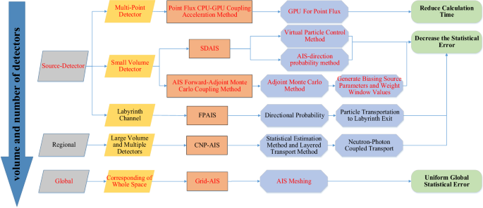
AIS-based Radiation Shielding Reduced Variance System.
Examples of spent fuel storage scenarios
As many nuclear power plants have begun to use the dry method for spent fuel storage, it is necessary to construct spent fuel storage system facilities for the away-from-reactor storage of spent fuel. Taking a dry process spent fuel transfer container as an example, this paper constructs a simplified arithmetic example under the spent fuel storage scenario to further create the above simulation dataset.
In this example, the calculation area is a cubic room with a side length of 10000 mm. Moreover, the thickness of the surrounding walls is 200 mm, and the material is concrete. The whole room is divided into two sides by a 200 mm wall. A spent fuel transfer container is placed vertically inside the room. The outer diameter of the container is 2340 mm, the inner diameter is 2200 mm, the height is 5000 mm, the bottom thickness is 200 mm, the container lid is 2400 mm, the height is 200 mm, and the container is made of stainless steel. At the same time, a cylindrical room beam with a diameter of 1000 mm and a height of 5800 mm is placed above the inner room to increase the geometric complexity. In this calculation example, the positions and coordinates of the main geometry are given in Table 1, and the geometric diagram is shown in Fig. 2.
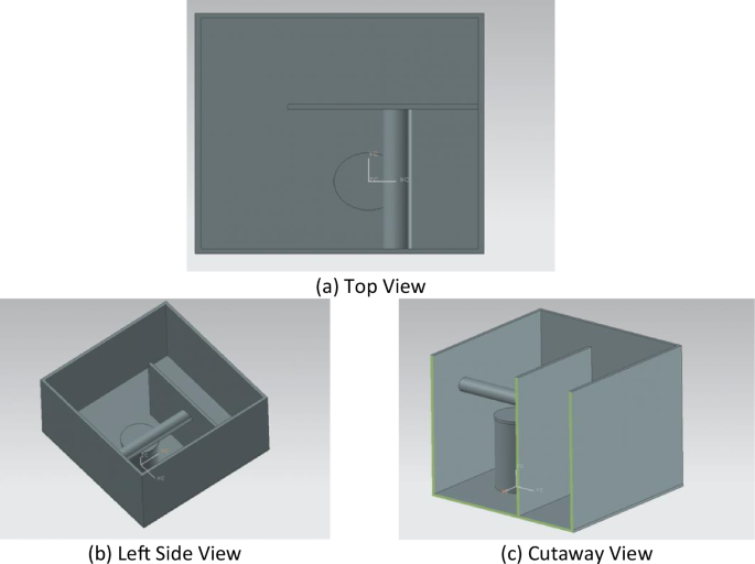
Geometry of a Simple Example of a Spent Fuel Transfer Container.
Examples of small modular reactors
Characterized by high safety, small size and multipurpose features, nuclear power plants have become faster and cheaper to build and safer to operate, and small modular reactors are becoming a future development trend for nuclear power. Based on a common small reactor design, this paper constructs a simulation dataset by using complex geometric examples of small reactors.
In this example, the calculation area is a rectangular room, with a length, width and height of 15400 mm, 12400 mm and 12400 mm, respectively. The coordinates of the lower left corner are (−4200, −4200, −1200). Moreover, the thickness of the surrounding walls is 200 mm, and the material is concrete. Shielding wall 1 is at (100, 10000, 12200). Shielding wall 2 is at (2100, 100, 12200). For Beam 1, the diameter is 200 mm, and the height is 8000 mm. For Beam 2, the diameter is 200 mm, and the height is 8000 mm.
The reactor was placed in a rectangular room. The reactor has an outer diameter of 2000 mm, a thickness of 100 mm, a height of 3000 mm, a hemispherical lower part, and four 300 mm diameter pillars made of stainless steel. A pressure vessel cover with a diameter of 3500 mm and a height of 500 mm is placed on the upper part of the reactor pressure vessel, which is made of stainless steel, and two main pumps with a height of 1600 mm and ten steam generators with a height of 850 mm are placed on the upper part, which are finally connected to two pressurizers with a diameter of 1500 mm and a length of 3500 mm to increase the complexity of the geometry. In this calculation example, the position and coordinates of the main geometry are given in Table 2, and the geometric diagram is shown in Fig. 3.
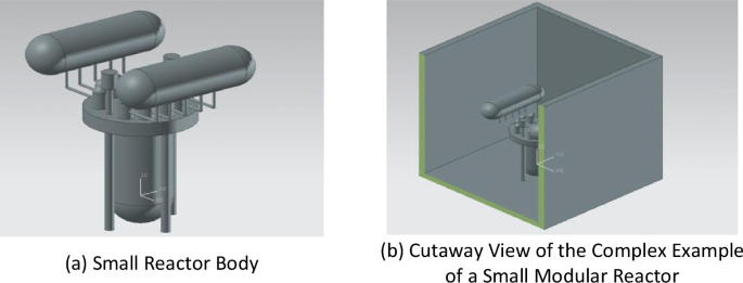
Geometry of the Complex Example of a Small Modular Reactor.
Monte carlo simulation parameter setting
In the calculation example presented in the article, the source term is defined as a custom neutron source with a Watt fission spectrum. During the simulation process, since nuclear facility containers are typically cylindrical in shape, the outer surface of the container can be treated as a curved source term. The surface intensity of the container exterior is utilized as the source strength, which allows the two-dimensional source term to be abstracted into a two-dimensional array. This array is characterized by two dimensions: the discretized circumferential angles and the axial discretized grids of the source term. As a result, the curved source term within the example is discretized into a series of subcurved sources for the purpose of the simulation. During the Monte Carlo simulation, the source term particles are uniformly ejected outward in the region with a certain intensity, assuming that the energy spectrum does not change. In the example described in this paper, the entire cylindrical container has a total of 360 degrees, which is divided into 30 angles for sampling. Each angle is divided into 20 regions for sampling, as shown in Fig. 4. For each example, 10,000 sets of examples are calculated as datasets. The number of simulated particles is 10000000, and the average statistical error is approximately 0.07. The MESH method is used to count the neutron flux in the whole calculation area, the side length of the MESH grid is 160 mm, and 64 MESH grids are set along the X, Y, and Z directions.
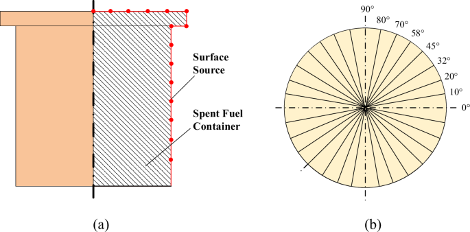
Complex Surface Diagram of the (a) Axial Mesh and (b) Circumferential Discrete Angles.
In this article, the 2D array above represents the strength of the discrete mesh for each source term. In the example, the intensity distribution of the source term is in the form of a 2D trigonometric function. When a set of source term distributions is generated, the parameters in the function are randomly sampled, including the series, amplitude, frequency and phase of the trigonometric function, and then the circumferential and axial coordinates of the source term are substituted into the 2D distribution function obtained by sampling to generate a set of source term parameters. To make the intensity distribution of the generated source term change continuously in both the circumferential and axial directions, a binary function is used to represent the source term intensity of each mesh, and a plurality of trigonometric functions with random parameters are used to represent the change trend of the source term intensity. The formulas are shown below:
$$F\,(x,y)\,=\sum _{{order}}\begin{array}{c}[{am}{p}_{1}\cdot \sin \,({fre}{q}_{1}\cdot x+{\varphi }_{1})\,+{am}{p}_{2}\cdot \cos \,({fre}{q}_{2}\cdot x+{\varphi }_{2})\,\\ \,+{am}{p}_{3}\cdot \sin \,({fre}{q}_{3}\cdot y+{\varphi }_{3})\,+{am}{p}_{4}\cdot \cos \,({fre}{q}_{4}\cdot y+{\varphi }_{4})\,],\end{array}$$
In this context, F(x, y) represents the source intensity at the circumferential grid x and the axial grid y. The parameters order, amp, freq, and φ are sampled randomly within a specified range according to a certain rule for each dataset generation. The sampling rules and ranges for these parameters can be customized each time the dataset is generated. For instance, the sampling conditions for the parameters in the dataset shown below are set as follows: order ∈ [1, 5], amp ∈ [1, 5], freq ∈ [0.001,0.5], and φ ∈ [−5,5]. Figure 5 below illustrates examples of two-dimensional distributions for different source terms in the dataset.
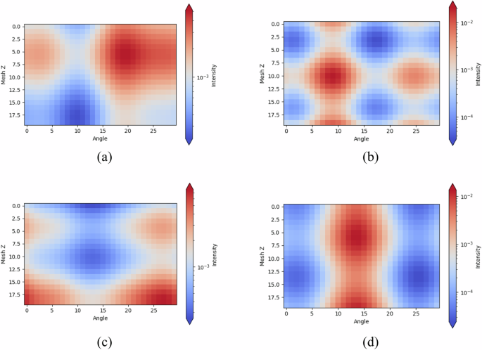
2D Distributions of the Source Terms for Different Generated Datasets.


