Towards a standardised methodology of radiation damage defect distributions for microstructure evolution models

The model presented here combines a database of primary damage configurations obtained through MD simulations with the PKA distribution given by a BCA code to generate the material damage produced by highly energetic ions in an efficient way.

We focus our research on self-ion irradiation of Fe and W, both corresponding to body-centered cubic (bcc) crystal structures, since they are widely used and because of our particular interest in fusion reactor structural materials. Therefore, the parameters and results below correspond to them.

Binary collisions approximation code

For the BCA component of our model, we utilise SRIM^31,32,33, a commonly used programme to calculate the NRT-dpa as a function of depth and determine the range of implanted ions.

We have developed a set of Python scripts that converts all SRIM output files (including those not used in this study) into a single SQLite database, organising each file into a separate table. This standardisation simplifies data extraction, filtering, and manipulation compared to the original, less structured text files. Additionally, the database format improves processing efficiency by eliminating the need for repeated string-to-numeric conversions required when reading text files.

SRIM users should be aware of its limitations and best practices. According to Agarwal et al.³⁴, the full-calculation mode should be used, since it employs more accurate stopping powers than the quick-calculation, especially for compound targets or for cases where the irradiation ion species is different from the target component(s) (\(Z_1 \ne Z_2\)). However, we have used the quick-calculation for multiple reasons. First, we are interested in simple materials and self-ion irradiation. Secondly, for the primary ions, the stopping powers are the same as for the full-calculation. Finally, we are only interested in the PKA distribution produced by the incident ions, and since the full-calculation mode follows all recoils (secondary, tertiary, etc.) these computations would not be used, so the quick-calculation is more efficient. Nonetheless, the full calculation recommendation must prevail for other cases.

We use the output file called COLLISION.txt (type “A”³²) to obtain the positions and energies of all PKAs produced by an ion, and then use them to evaluate the dpa models and as input for our model. Since SRIM does not store the PKA direction and is required by our algorithm (“Algorithm”), we need to apply some approximation to calculate it. We have chosen a simple solution: the PKA direction is given by the PKA position minus the previous PKA position (this is further discussed in appendix B in the Supplementary Material).

Table 1 presents a summary of the input parameters used in our model calculations, including those applied in SRIM.

Damage energy calculations

As described above, from SRIM we obtain the PKA energies of each ion as it travels through the material. The PKA energy is the total energy transferred to the PKA and includes the energy that will be lost in inelastic collisions that, as mentioned in³⁴, has to be subtracted to obtain the damage energy. In our case, the damage energy is needed to compare the results of our method with the dpa models described above. This implies the need to establish a relationship between \(T_{dam}\) and \(E_{PKA}\). The Lindhard equation (2) is not suitable for comparisons with MD simulations, as demonstrated by Sand et al.³⁵, who observed discrepancies in \(T_{dam}\) calculations, particularly at high energies and low atomic numbers. Furthermore, in MD, the electronic stopping friction term depends on parameters that vary between researchers, typically derived from SRIM.

There are, however, multiple methods to derive this relation from SRIM^34,36,37, often yielding different results. To our knowledge, this relation has only been explicitly published for Fe self-ion irradiation in³⁸. In our case, we have determined this relation using SRIM, following the different methods proposed in³⁴ with their recommended parameters (see Table 1). The ions are initiated at some depth and the target is wide enough to avoid backscattering and transmission, since this could lead to the modification of the equations calculation of the damage energy³⁶.

Among the approaches tested, the D1 method³⁴ in quick-calculation mode has shown a better agreement with the MD database used (see “Molecular dynamics database”) when comparing to the fer-arc-dpa than the fit from³⁸ or other calculations for Fe. Therefore, we also use this method for W.

The relation \(T_{dam}\left( E_{PKA}\right)\) is obtained using a least-squares fit to a second-degree polynomial expression:

where \(E_{PKA}\) and \(T_{dam}\) are in keV. The errors correspond to the standard deviation errors given by the fit.

Damage energy as a function of PKA energy for Fe (1a ) and W (1b ). The black dots are obtained using SRIM in quick-calculation mode with the parameters recommended by³⁴ following the D1 method. A second-degree polynomial fit to these data points is depicted by the black line. The orange line corresponds to the Lindhard equation (Eq. (2)). The blue line is the relation provided in³⁸ for Fe.

If we compare the results with the Lindhard Eq. (2) (see Fig. 1), in the case of Fe, the new damage energy relation is above the former, as in³⁵ for Ni (similar atomic numbers), although it must be noted that the methodologies are different but based on SRIM. For W, the results are almost identical, as occurs with Pt³⁵.

Molecular dynamics database

In our approach, the defects produced for a given \(E_{PKA}\) will be extracted from MD simulations of collision cascades. Consequently, we need a database of cascade debris. We have used CascadesDB (https://cascadesdb.iaea.org/), as it is an easily accessible source of simulations. One advantage of using this database is that it includes calculations with electronic stopping as a frictional force for all atoms with kinetic energies above a given threshold. This is crucial since the BCA programme we use (“Binary collisionsapproximation code”) provides us with the PKA energy and not the damage energy, so we do not have to rely on formulas for its calculation.

CascadesDB provides the final positions of all atoms. Therefore, to extract the information needed for our purposes, which is the position of the defects at the end of the collision cascade, we have implemented a modified version of the defect identification algorithm proposed by Bhardwaj et al.³⁹, detailed in the appendix A in Supplementary Material. The vacancies and self-interstitials identified with this algorithm are what we call the cascade debris.

In Tables 2 and 3, the number of CascadesDB bulk samples are listed for Fe and W, respectively. Since the database contains cascade damage simulated with different interatomic potentials, which have different equilibrium lattice constants, the lattice parameter used when placing the debris is scaled if needed to match that given in Table 1. A further difference between the data found in the database concerns electronic stopping, which was introduced in all simulations for kinetic energies greater than 10eV, except for the ones in reference⁴⁰ whose threshold is 1eV. We do not expect notable differences at these low PKA energies as occurs with other metals³⁵. We have access to energies up to 200 keV with significant statistics (especially for W). However, as will be noticed later, the separation between energies is sometimes too high, and we will need to apply some approximation to get intermediate points (“Energy decomposition”).

In Fig. 2, the number of displaced atoms for each energy in the database and its comparison with the fer-arc-dpa prediction is plotted. The damage energy is derived from Eqs. (10) (Fe) and (11) (W). It can be seen that for iron, the number of displaced atoms fits approximately the fer-arc-dpa model. On the other hand, in the case of tungsten, there is a notable discrepancy at energies greater than 50 keV. In fact, in the arc-dpa original work²⁵ a discrepancy is already observed for the highest energies (notice that the x-axis in Fig. 2 is the PKA energy, while in²⁵ it is the damage energy). From the analysis of the defects formed at the highest energies in W from the MD database, we have observed the formation of large clusters that appear to impede recombination and subcascade splitting (see Fig. 3b ). This was previously reported by Sand et al. in^41,42 for 150 keV. A visual representation of a cascade of 200 keV for each material is shown in Fig. 3.

Number of displaced atoms from CascadesDB simulations of Fe (2a ) and W (2b ). The black line is the fer-arc-dpa model prediction and the orange dots are the number of displaced atoms from CascadesDB simulations. To convert the PKA energy into a damage energy to evaluate the fer-arc-dpa model, Eqs. (10) (Fe) and (11) (W) are used. The error bars are calculated as the standard error of \(N_d\) for each PKA energy.

Examples of debris from the MD cascade database of 200 keV for Fe (3a ) and W (3b ). SIAs and vacancies are represented as red and blue spheres, respectively. The PKA is initiated from the left. Scale and sphere radius was adapted for each image in order to visualise defects more easily. Images generated with OVITO ⁴⁴.

The cluster size distribution in the database is represented in Fig. 4. We have implemented a cluster recognition code based on the union-find data structure as in⁴³ (first stage) that has been tested with OVITO⁴⁴ cluster identification to verify its results. Two defects are considered to belong to the same cluster if their distance is smaller than or equal to the third nearest neighbour for SIAs (self-interstitials atoms) (\(\sqrt{2}a_0\) for a bcc lattice) and the second for vacancies (\(a_0\))^10,45. The missing bins for each energy suggest that we need more simulations to have a complete representation of all possible cluster sizes.

Defect cluster size distribution for the PKA energies available in CascadesDB for Fe (4a ) and W (4b ). Counts are normalized to the number of simulations for each energy.

Energy decomposition

We now need to combine the PKA energies of each ion obtained with SRIM with the MD defects from CascadesDB. However, most of the PKA energies given by the BCA code will not correspond to a given energy in the database of MD simulations; they will be either higher in energy than the highest in the MD database or of an energy not included. To overcome this limitation, we have performed almost the same approximation as Adjanor et al.⁴⁶. If the set of energies in the database is denoted as \(\mathcal {E}^{MD}=\{E^{MD}_{i}\}_{i}\) in descending order, then the PKA energy, \(E_{PKA}\), is projected into this base:

where \(n_i\) are positive or null integers and \(\Delta E\) is what we have called the residual energy. To calculate \(n_i\), an iterative procedure must be followed. First, for the highest energy: \(n_1 = \left\lfloor E_{PKA}/E^{MD}_1\right\rfloor\) (floor/integer division). The rest of the coefficients are given by

Using this approach we ensure that the highest energies in the MD database are used first and we are also able to obtain the number of collision cascades needed for the different energies.

Finally, Eq. (12) is used to get \(\Delta E\). Therefore, the code randomly chooses \(n_i\) cascade debris of energy \(E_i^{MD}\) for each i and uses the fer-arc-dpa model to get the number of Frenkel pairs equivalent to the residual energy \(\Delta E\). In “Algorithm” we will discuss where to place defects.

One more detail must be taken into account. For highly energetic ions, there will be PKA energies well above the database limit. In order to address this issue and avoid using many debris of the highest energies in the database, we have implemented a code to be able to run SRIM iteratively: for all PKA energies above a given threshold (\(E_{PKA}^{max}\)), SRIM is run again until the resulting PKA energies are below this value. For the cases presented here we have chosen \(E_{PKA}^{max}={250}{\,\text {keV}}\) for Fe and W, which is above the maximum PKA energy in the MD database. We have also tested the case for Fe where a lower value is used, \(E_{PKA}^{max}={35}{\,\text {keV}}\), which is around the energy threshold when subcascades begin to form²⁷. In this case, SRIM will have to run iteratively more times and only low-energy cascades from the database will be used, eliminating the chances of phenomena that occur only in highly energetic cascades, such as the formation of certain defect clusters.

Algorithm

The following is the step-by-step process of our model to obtain the defects produced by highly energetic ions, which is automated by our code and schematically represented in Fig. 5 and in the flow diagram of Fig. 6:

1. 1.

   Simulate multiple ions with SRIM (usually ten thousand) and run it iteratively until all PKA energies are below \(E_{PKA}^{max}\) (see “Energy decomposition”).

2. 2.

   For each ion, for each PKA, apply the energy decomposition, Eq. (12). Denote \(i=I\) as index corresponding to the highest energy in \(\mathcal {E}^{MD}\) with \(n_i \ne 0\).

   • If I exists:

     1. (a)

        Take the debris from a cascade (obtained from the MD data as described in “Molecular dynamics database”) chosen randomly among the ones available in the database for the energy I. Place those debris in the PKA position with the corresponding direction, selected as described in appendix B in Supplementary Material.

     2. (b)

        Define a parallelepiped containing all the defects of the cascade debris of (a).

     3. (c)

        If there are further cascades that are needed to be included for that given PKA energy, that is, if there are coefficients \(n_i \ne 0\), select \(n_i\) cascades at random from the MD database for the corresponding energy. For each cascade select a location at random within the parallelepiped and place the debris in that position.

     4. (d)

        For the residual energy, \(\Delta E\), first use Eqs. (10) (Fe) or (11) (W) to get the damage energy. Then apply Eq. (9) to get the corresponding number of displaced atoms (round the result to get an integer number). Place them randomly inside the parallelepiped as Frenkel pair (FPs) (the distance between the SIA and vacancy is \(4a_0\)).

   • Else (PKA energy too low for the database, only residual energy, \(\Delta E\)):

     1. (a)

        First, use Eqs. (10) (Fe) or (11) (W). Then apply Eq. (9) to get the corresponding number of displaced atoms (round the result to get an integer number). Place them randomly in a sphere situated at the PKA position plus its direction multiplied by the radius of the sphere. The radius of the sphere is the length occupied by all FPs if they were aligned in a straigth line.

Note that the relation between the PKA and the damage energies is only used in low energy collisions, therefore, despite the ambiguities, we do not expect significant changes if another methodology to determine that relation is used.

Scheme of the algorithm proposed. The yellow arrows represent the trajectory of the PKA, the red and blue spheres are SIAs and vacancies, respectively, forming FPs; and the blue-red ellipses correspond to MD debris.

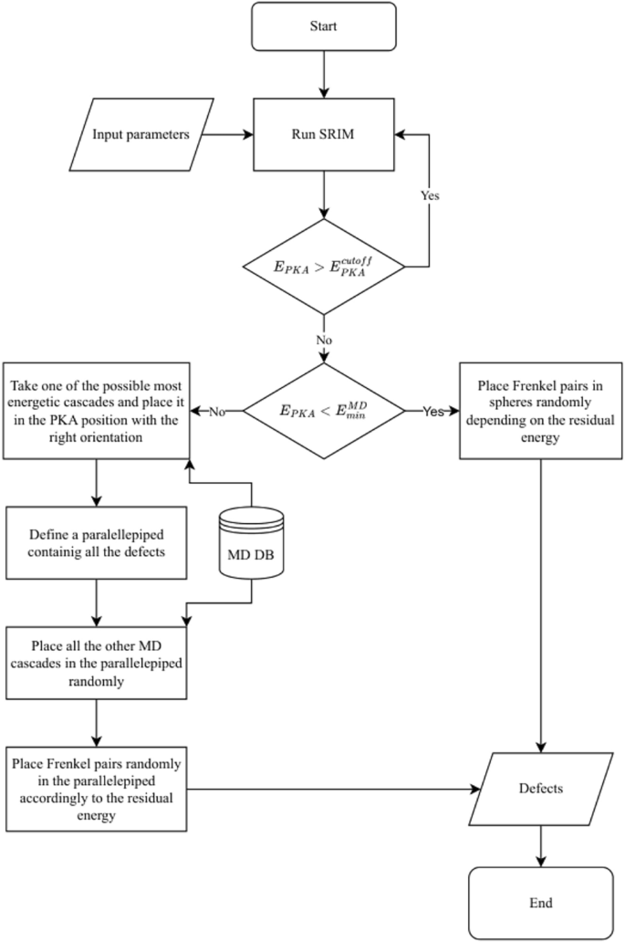
Flow diagram of the algorithm proposed.

Evaluation

Once the algorithm is established, it is required to evaluate it in order to determine its validity and accuracy. We have compared the results of our model with those provided by the NRT-dpa and fer-arc-dpa models, and the CascadesDB database. We will refer to the dpa given by our methodology as debris-dpa for easy reference.

Firstly, we have used our model to simulate the damage generated by PKAs of all energies in the MD database both for Fe and for W to compare with the results of the full MD simulations. For Fe, we have tested two scenarios: \(E_{PKA}^{max}={35}{\,\text {keV}}\) and \(E_{PKA}^{max}={250}{\,\text {keV}}\). The results are depicted in Fig. 7, comparing also with NRT-dpa and fer-arc-dpa.

Predicted number of displaced atoms for different models: fer-arc-dpa (black line), NRT-dpa (orange line), CascadesDB database (blue dots), debris-dpa for \(E_{PKA}^{max}={250}{\,\text {keV}}\) (green dots joined by a line), and the debris-dpa for \(E_{PKA}^{max}={35}{\,\text {keV}}\) (yellow dots joined by a line, only for Fe). The error bars are calculated as the standard error of \(N_d\) for each PKA energy.

In the case of Fe, it is observed that when \(E_{PKA}^{max}={35}{\,\text {keV}}\) more displaced atoms are produced than in the case with \(E_{PKA}^{max}={250}{\,\text {keV}}\): since more iterations are required, there will be more PKAs given by SRIM of low energy, removing the chances of recombination and clustering. In both cases \(N_{d}\) is somewhere between the fer-arc-dpa and NRT-dpa models, being significantly closer to the former.

W remains a particular case due to its deviation from the fer-arc-dpa model, as noticed in Fig. 2b . However, the prediction for \(N_{d}\) still falls between the fer-arc-dpa and NRT-dpa models, getting a decent agreement with the MD prediction.